Downscaled Climate Projections
Statistical Models - Temperature
Summary
We use linear regression to predict the temperature given large-scale atmsopheric state. We add gaussian noise to the linear fit to simulate the portion of the variance that is unexplained. In some cases, we allow the variance of the noise to vary with the predictors even though the assumptions of linear regression do not strictly hold in this case.
Linear Regression
The most basic model for relating a dependent variable to independent variables is linear regression. The linear regression model takes the form \begin{equation}\label{eqn:lin_regr} y(t) = a_0 + a_1x_1(t) + a_2x_2(t) + \ldots \end{equation} where $a_i$ are constants that are usually obtained by minimizing the sum of the squared 'errors' between $y(t)$ and the value of $y(t)$ predicted from $x_i(t)$. Written in mathematical form, we find the $a_i$ that minimize \begin{equation}\label{eqn:sq_err} \epsilon = \frac{1}{T-1} \sum_{t=1}^T{\left( y(t) - a_0 - a_1x_1(t) - a_2x_2(t) - \ldots \right) }^2 \end{equation} where $\epsilon$ denotes the error and $T$ is the total number of times in the statistical sample. In linear regression, we predict the mean of $y(t)$ given the $x_i(t)$, but as mentioned previously, we must know how $y(t)$ deviates from this mean in order to capture the variability and extremes in $y(t)$. According to classical linear regression theory, the errors from the mean are distributed in a normal distribution with a variance of $\epsilon$. Thus, the full Probability Density Function (PDF) of $y(t)$ contingent on $x_i(t)$ is: \begin{equation}\label{eqn:lin_regr_norm} \Pr { \left\{ y(t) = z \right\} } = \frac{1}{\sqrt{2\pi}\sigma}\exp\left(-\frac{(z-\mu(t))^2}{2\sigma^2}\right) \end{equation} where $\mu(t) = a_0 + a_1x_1(t) + a_2x_2(t) + \ldots $ and $\sigma^2 = \epsilon$. Note that the standard deviation, $\sigma$, of the normal distribution in equation (\ref{eqn:lin_regr_norm}) is a constant and therefore completely independent of the variables $x_i(t)$. Also note that the minimization of the error in equation (\ref{eqn:sq_err}) can be applied to any data, but only for normally distributed errors are these 'least squares' estimates of $a_i$ the most likely estimates given the data.
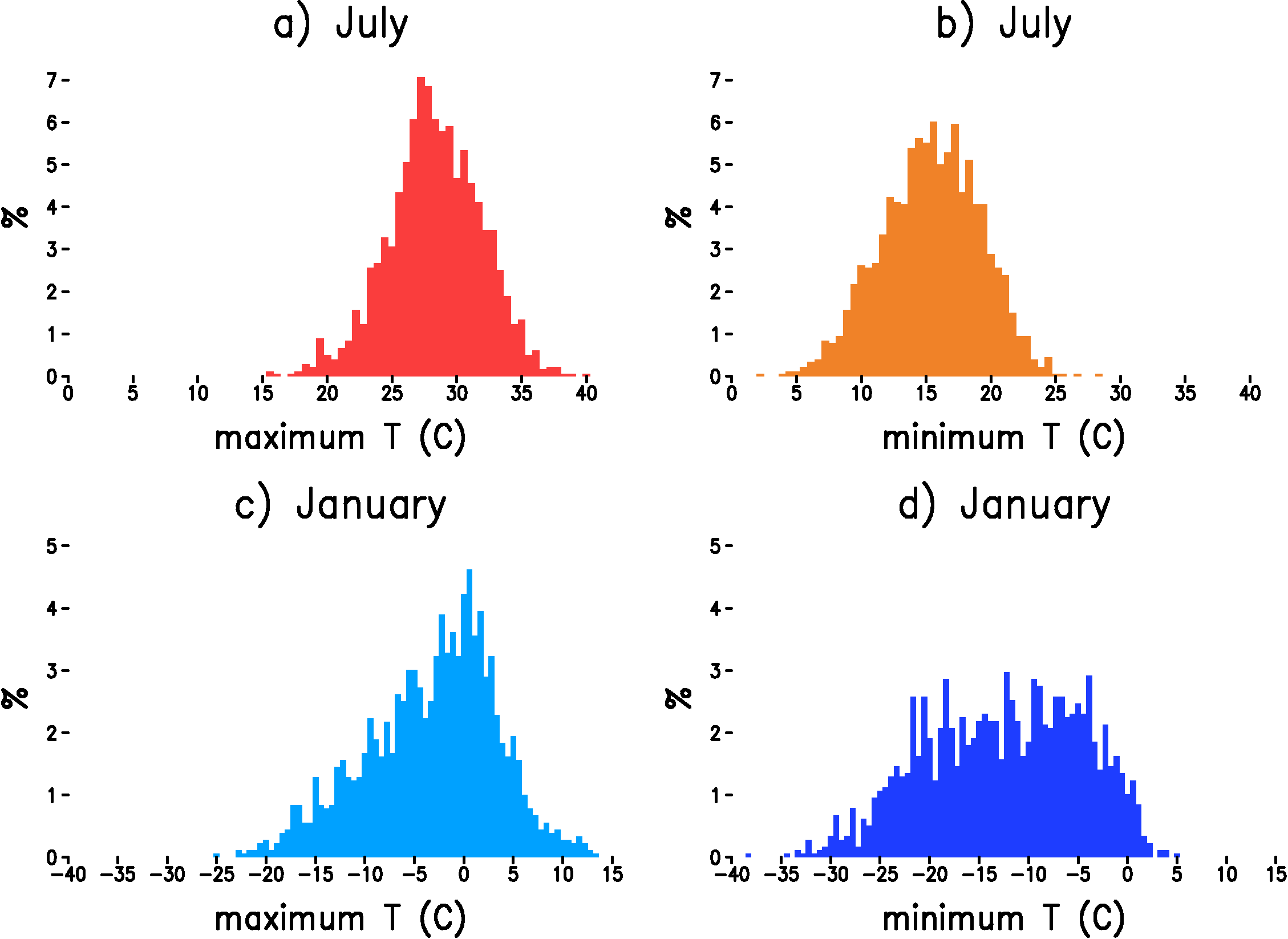
Figure 1: Histogram of daily maximum or minimum temperature at Madison, WI. a) maximum temperature in July. b) minimum temperature in July. c) maximum temperature in January. d) minimum temperature in January. The y-axis is the number of days in each bin divided by the total number of days (%) and the x-axis is the temperature at the bin center in Celsius. The bin width is 5/9 degrees.
Because the distributions maximum and minimum temperature are continuous with no obvious sharp bounds on the range of possible values, linear regression and the assumption of normally distributed errors might be a reasonable model for these two variables. Looking at the histogram of daily maximum and minimum temperature for Madison, WI in July, we see that the distribution generally follows our notion of the symmetric, 'bell curve' shape of the normal distribution (Figure 1). In January, however, the distribution of maximum temperature is noticeably skewed toward cold days and the distribution of minimum temperature seems excessively broad and flat in relation to the normal distribution. Before giving up on classical linear regression, however, we must note that the errors must be normally distributed not the actual values of the dependent variable. If the large-scale independent variables also exhibit the departures from normality seen in Figure 1, then there is hope that the errors might actually be close to normally distributed. Looking at the histogram of the large-scale maximum daily temperature, we indeed see that the large-scale temperature shows similar departures from normality as the record at Madison, WI (Figure 2a).
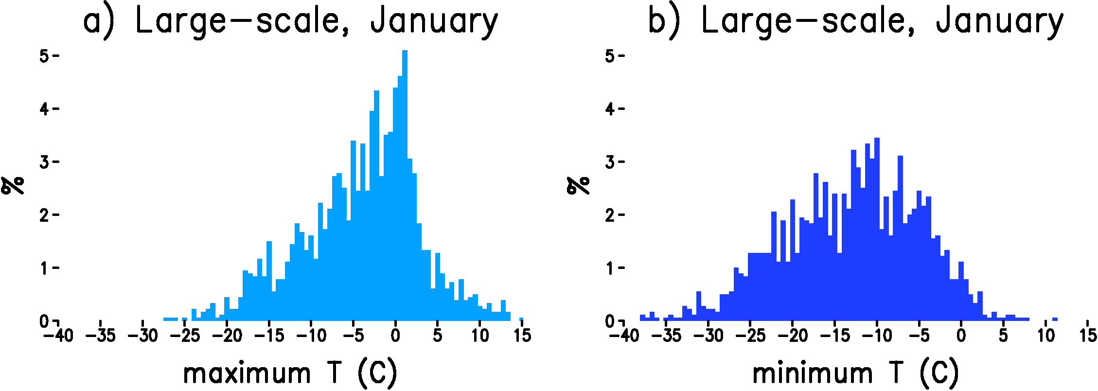
Figure 2: Histogram of daily maximum or minimum temperature at the grid point in the NCEP Reanalysis closest to Madison, WI. a) maximum temperature in January. b) minimum temperature in January. The y-axis is the number of days in each bin divided by the total number of days (%) and the x-axis is the temperature at the bin center in Celsius. The bin width is 5/9 degrees.
It turns out that linear regression gives an excellent fit to the observed PDF of maximum temperature in January. For minimum temperature in January (Figure 2b), however, the distribution of the large-scale from the NCEP Reanalysis is not as flat in the middle as the observed histogram and the upper tail of the distribution is too pronounced for the large-scale. Another problem with linear regression for minimum temperature in winter, which is not evident here, is the assumption of constant variance. We find that the standard deviation, $\sigma$, in equation (\ref{eqn:lin_regr_norm}) is not constant, but depends on $x_i(t)$. While, we still use linear regression to predict the mean, $\mu$, minimum temperature in winter, we implement additional corrections described in detail below so that the downscaling of the extremes in minimum temperature are much better represented.
Non-constant Variance
Under Construction
Home