Downscaled Climate Projections
Statistical Models - Precipitation Occurrence
Summary
We use logistic regression to predict the probability that there is non-zero precipitation given the large-scale atmsopheric state.
Logistic Regression
To model the relationship between large-scale variables and the occurrence of precipitation at a point, we use a broader class of statistical models than linear regression known as generalized linear models. A generalized linear model consists of three components:
- A distribution function from the exponential family (includes the normal, binomial, Poisson, gamma, and Weibull distributions)
- A linear predictor $\eta(t) = a_0 + a_1x_1(t) + a_2x_2(t) + \ldots$
- A link function $g$ such that ${\rm E}(y) = \mu = g^{-1}(\eta)$, where ${\rm E}(y)$ denotes the expected value, or mean, of $y$.
For classical linear regression the distribution function is the normal distribution and the link function is the identity function so that ${\rm E}(y) = \mu = \eta = a_0 + a_1x_1(t) + \ldots$ .
In our precipitation occurrence model the value of "precipitation occurrence", $P_{occ}$, takes one of two values \begin{equation}\label{eqn:p_occ} P_{occ}= \begin{cases} 1, & \textrm{if the day is wet,} \\ 0, & \textrm{if the day is dry.} \end{cases} \end{equation} We predict the probability, $\mu$, that the day is wet. Obviously $\mu$ should be between 0 and 1 inclusive. The generalized linear model that corresponds to binary data such as $P_{occ}$ has a special name: logistic regression. The 'canonical' inverse link function for logistic regression is the logistic function \begin{equation}\label{eqn:logistic} \mu = g^{-1}(\eta) = \frac{1}{1+\exp(-\eta)} \end{equation} where $\eta = a_0 + a_1x_1(t) + a_2x_2(t) + \ldots$ as before. The logistic function approaches 0 as $\eta \rightarrow -\infty$ and the function approaches 1 as $\eta \rightarrow \infty$ (Figure 1). (Note, we find it much easier to think in terms of the inverse of the link function, $g^{-1}$, rather than the link function itself.)
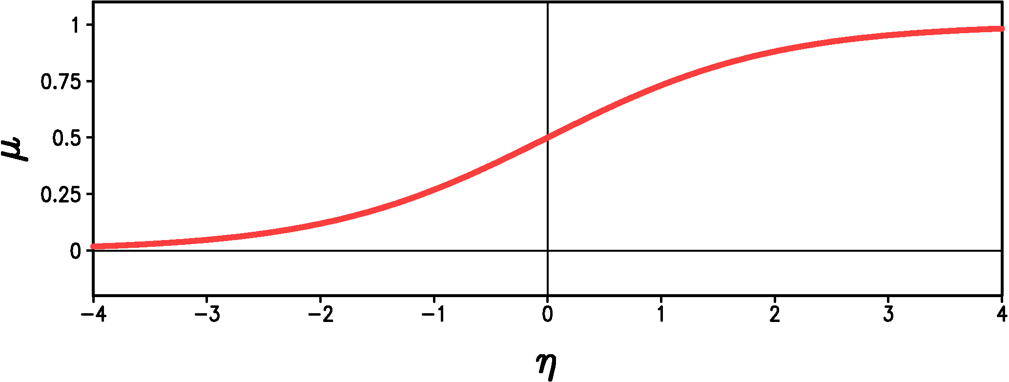
Figure 1: Graph of the logistic function (Equation \ref{eqn:logistic}).
Regardless of the values of the dependent variables, $\mu$ always lies on the interval from 0 to 1 just like a probability should. The logistic regression model is fit by the method of maximum likelihood, which finds the constants $a_i$ that make up the expression for $\eta$. After we fit the model, we can calculate $\eta$ from the large-scale predictors, $x_i(t)$. We then transform $\eta$ to get the probability of precipitation, $\mu$, using equation (\ref{eqn:logistic}). To generate a time series of $P_{occ}$ we generate a time series of uniformly distributed random numbers between 0 and 1, $r(t)$. If $r(t) < \mu(t)$, then the day is wet, otherwise the day is dry.
One is also free to choose other links relating $\mu$ to $\eta$ besides equation (\ref{eqn:logistic}), but we have found that the logistic link works just as well or better than the other links we have tried.
Home