Downscaled Climate Projections
Statistical Models - Precipitation Amount
Summary
We use a generalized gamma distribution conditioned on the large-scale atmsopheric state to predict the preciptation amount if a day has non-zero precipitation. We describe the reason for using this more complicated distribution below.
A Potential Model for Precipitation Amount on Wet Days
As shown previously, the daily precipitation amount on wet days is strongly skewed toward large precipitation amounts while the most likely amount is the smallest measurable value. Hence a potential distribution for precipitation amount on wet days, $P_{am}$, that fits within the generalized linear model framework is the exponential distribution: \begin{equation}\label{eqn:p_am_exp} \Pr { \left\{ P_{am}(t) = z \right\} } = \begin{cases} \frac{1}{\mu(t)}\exp\left(-\frac{z}{\mu(t)}\right), & z>0 \\ 0, & \textrm{otherwise} \end{cases} \end{equation} where $\mu$, the mean value of the distribution, must be positive. Because $\mu$ is constrained to be positive, we should use an inverse link function that automatically satisfies this constraint. One such link function is the exponential function, $\mu = \exp(\eta)$ (Figure 1).
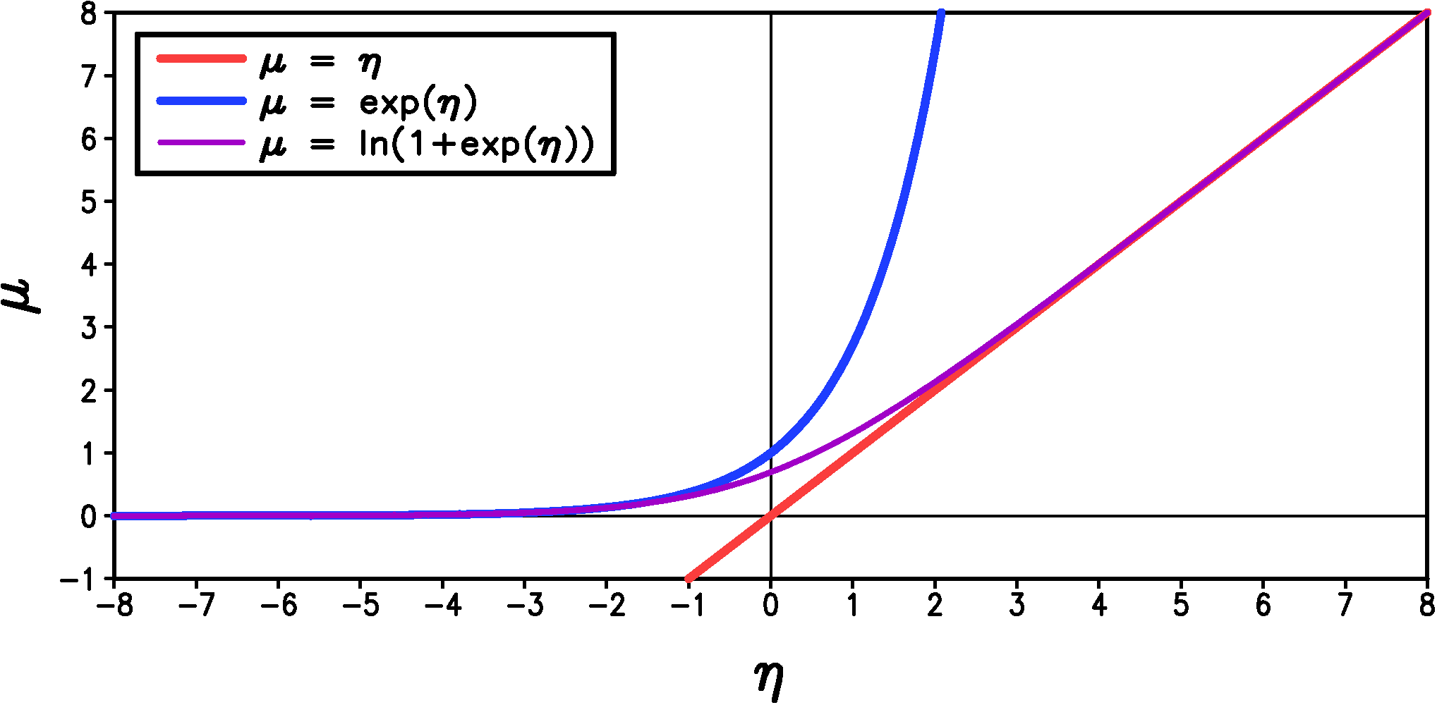
Figure 1: A plot of potential inverse link functions for 'exponential' regression.
Unfortunately, we have good reasons to believe that the mean of the station precipitation should increase linearly rather than exponentially with our large-scale predictors, especially because large-scale precipitation itself is one of the potential predictors. The problem with the linear or identity link ($\mu = \eta$) is that it is not constrained to be positive for all $\eta$ (see the red line in Figure 1). To avoid the problems associated with non-positive $\mu$ for the identity link, we devise a new link which is close to the identity link for $\eta>0$ but which transitions to the exponential link when $\eta<0$. The functional form of this link is \begin{equation}\label{eqn:qlinear} \mu = \alpha\ln\left(1+\exp\left(\frac{\eta}{\alpha}\right)\right) + \beta \end{equation} where $\alpha$ is a constant that controls how quickly the function transitions from exponential to linear (small $\alpha$ gives a faster transition). We also have an additional parameter $\beta$ which is typically a very small positive number. This prevents the mean from becoming arbitrarily close to zero which is inconsistent with the fact that the measured precipitation data has a smallest non-zero value of 0.254 mm (for US data). The new link is shown in Figure 1 for $\alpha = 1$ and $\beta = 0$. We call this new link the quasi-linear link and we denote it by angled brackets so that is looks more like the identity link, to which it is very close over most of the range of $\eta$ in our statistical fits to the data: \begin{equation}\label{eqn:qlinear2} \textrm{'quasi-linear' link: } \mu = \langle \eta \rangle = \alpha\ln\left(1+\exp\left(\frac{\eta}{\alpha}\right)\right) + \beta \end{equation}
The exponential model is fit by the method of maximum likelihood. To generate a time series of precipitation, we first use the random precipitation occurrence time series created previously. If this random time series indicates that a particular day is wet, then we generate an exponentially distributed random number with a mean $\mu$ to represent the amount of precipitation for that day. Remember that the mean for the exponential distribution, $\mu$, depends on time.
Unfortunately, exponential regression tends to over-predict the extremes when applied to observed precipitation data. We explore the reason why below.
Beyond Generalized Linear Models
Even though the most likely value for $P_{am}$ is the smallest measurable value when considering all wet days together, the $P_{am}$ distribution may not necessarily have this form when we limit the days to times when the large-scale atmosphere is in a particular state. For example, consider the case of a large-scale predictor that is very strongly correlated with $P_{am}$. When this predictor is small we would expect the most likely $P_{am}$ to be close to zero, but when the predictor is large, it is certainly possible that the most likely value value of $P_{am}$ is also large. The exponential distribution (equation \ref{eqn:p_am_exp}) cannot capture this behavior because it has the same basic shape for all values of $\mu$.
To check if this scenario holds in our data, we first select large-scale precipitation as our predictor because we believe it has the most potential to explain the variations in $P_{am}$. We then rank the values of the predictor from smallest to highest and divide the days into 40 sets based on the value of the predictor. The days when the predictor is in the smallest 2.5% of its range get put in the first set, the days when the predictor is in the 2.5% to 5% part of its range get put in the second set, and so on until the the top 2.5% of predictor values. We then compute the precipitation amount histogram at the weather station for all the wet days in each set. The above procedure is done individually for each station in Wisconsin and vicinity, and then all the histograms are averaged together to smooth out the noise. The result of this analysis for the winter months (Dec.-Feb.) is shown in Figure 2 together with the best fit to the data using either the exponential or gamma distributions.
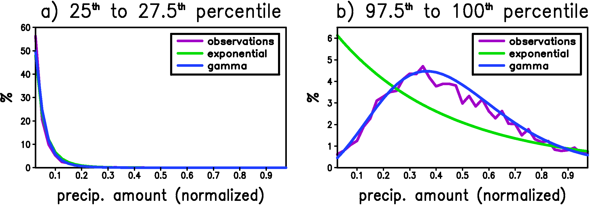
Figure 2: The histogram of precipitation amount when the large-scale predictor is in a) the 25th to 27.5th percentile and b) the 97.5th to 100th percentile. The histogram is an average over all stations. The best fit of the data to both the exponential and gamma distributions is also shown. These fits are performed individually for each station and the result shown is the average over these fits. The precipitation amount on the x-axis has been normalized at each station by dividing by the precipitation amount on the wettest day in the entire record for that station. The y-axis is the number of days in each bin divided by the total number of wet days occurring within the specified range of large-scale predictor. There are 40 bins.
For relatively small values of the predictor (25th to 27.5th percentile), the most likely value of precipitation is the smallest measurable value, and both the exponential and the gamma distribution can capture the general behavior of the histogram. For large values of the predictor, however, the most likely value for precipitation is significantly greater than the smallest measurable value. The exponential fit to the data has the correct mean, but to achieve this correct mean it over-predicts the number of weak events, under-predicts the middle range of events and, although it is not evident in Figure 2b, it over-predicts the extreme events. In fact, the over-prediction of the extreme events is the most obvious flaw of the exponential fit (equation \ref{eqn:p_am_exp}) when we consider the histogram of the entire data-set (i.e. all percentiles of the predictor together). The gamma distribution, on the other hand, is able to capture the shift of the most likely value of precipitation for large values of the large-scale predictor.
The Gamma Distribution
The gamma distribution achieves greater flexibility compared to the exponential distribution by having an additional parameter for a total of two parameters that specify the distribution: \begin{equation}\label{eqn:p_am_gam1} \Pr { \left\{ P_{am}(t) = z \right\} } = \begin{cases} \frac{1}{b\Gamma(a)} \left(\frac{x}{b}\right)^{a-1} \exp\left(-\frac{z}{b}\right), & z>0 \\ 0, & \textrm{otherwise} \end{cases} \end{equation} where $a$ is the `shape parameter', which must be greater than zero, $b$ is the `scale parameter', which must also be greater than zero, and $\Gamma$ is the gamma function, which is required here simply to make the integral of the PDF over all $z$ equal to one. As the shape parameter, $a$, increases the distribution becomes less confined to small values and for shape parameter greater than one the most likely value value becomes greater than the smallest measurable value (Figure 3).
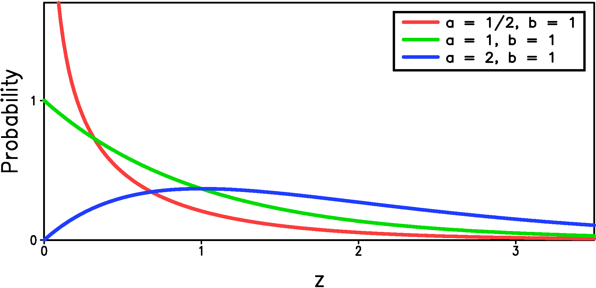
Figure 3: The gamma distribution (equation \ref{eqn:p_am_gam1}) for three different values of the shape parameter, $a$. The scale parameter, $b$, is one in all cases.
The gamma distribution reduces to the exponential distribution when $a=1$, and in this case the scale parameter, $b$, is also the mean, $\mu$. But for general $a$, the mean of the gamma distribution is $\mu = ab$. Because we expect the mean to depend linearly on the large-scale predictors, we rewrite the gamma distribution in terms of the mean and the shape parameter: \begin{equation}\label{eqn:p_am_gam2} \Pr { \left\{ P_{am}(t) = z \right\} } = \begin{cases} \frac{a}{\mu\Gamma(a)} \left(\frac{ax}{\mu}\right)^{a-1} \exp\left(-\frac{az}{\mu}\right), & z>0 \\ 0, & \textrm{otherwise.} \end{cases} \end{equation} In this statistical model we have $\mu$ and $a$ depend on the large-scale predictors through the quasi-linear link (equation \ref{eqn:qlinear2}): \begin{equation}\label{eqn:mu_a} \begin{split} a & = \langle \eta_{a} \rangle = \langle a_0 + a_1x_1(t) + a_2x_2(t) + \ldots \rangle \\ \mu & = \langle \eta_{\mu} \rangle = \langle b_0 + b_1x_1(t) + b_2x_2(t) + \ldots \rangle \end{split} \end{equation} Note that both $a$ and $\mu$ depend on time for our model, but we leave out the explicit time dependence in equation (\ref{eqn:p_am_gam2}) so that it is more readable. The gamma distribution model is fit by the method of maximum likelihood, which finds the constants $a_i$ and $b_i$ on the right side of equations (6).
This statistical model is not a generalized linear model even though the gamma distribution is a member of the exponential family of distributions. The reason is that the shape parameter must be independent of the predictors, $x_i(t)$, for generalized linear models, but we have found that the shape parameter varies significantly with the predictors (see Figure 2).
The Generalized Gamma Distribution
While the gamma distribution is an improvement over the exponential discussed previously, we find that it is not flexible enough to capture the extremes in precipitation. The gamma distribution can either over- or under-predict the extreme precipitation (depending on location or time of year) but it is more common for it to under-predict the extremes. To have more control over the decay of the distribution in the tails of the distribution we use the generalized gamma distribution: \begin{equation}\label{eqn:p_am_ggam} \Pr { \left\{ P_{am}(t) = z \right\} } = \begin{cases} \frac{c}{b\Gamma(\frac{a}{c})} \left(\frac{x}{b}\right)^{a-1} \exp\left(-\left(\frac{z}{b}\right)^c\right), & z>0 \\ 0, & \textrm{otherwise.} \end{cases} \end{equation} The key generalization in equation (\ref{eqn:p_am_ggam}) is the addition of $c$ in the term that determines the behavior of the distribution for large $z$: $\exp\left(-\left(z/b\right)^c\right)$. When $c < 1$ then the distribution has a 'heavier' tail that decays more slowly than the standard 'exponential-like' tail of the gamma distribution ($c = 1$). A heavier tail increases the extremes relative to the mean and will help correct the most common bias in the gamma distribution. Likewise a 'lighter' tail will help correct cases where the gamma distribution over-predict extremes.
We find that letting $c$ be a constant independent of time (unlike the other two parameters) allows enough flexibility to capture the extremes. This is advantageous because our limited sample size limits the number of the free parameters that we can estimate reliably. As in the case of the gamma distribution, we predict the mean, $\mu$, directly in terms of the predictors instead of the scale parameter, $b$. Unlike the gamma distribution, however, the formula for the mean is rather complicated: \begin{equation}\label{eqn:mom_ggam} \mu = b\frac{\Gamma\left(\frac{a+1}{c}\right)}{\Gamma\left(\frac{a}{c}\right)} \end{equation} The mean, $\mu$, and the shape, $a$, depend on the large-scale predictors in the same way as the gamma distribution (equation 6). After $\mu$ and $a$ are known, we use equation (\ref{eqn:mom_ggam}) to find $b$.
The procedure for estimating the parameter $c$ for the generalized gamma distribution is different than that for the other distributions. Because $c$ is meant to capture the extremes, which by definition are very rare, we do not estimate $c$ individually for each station like we do for the other parameters. Instead $c$ is fit region by region by aggregating at least 200 stations together. The details will be described later.
Home